F. Caubet, C. Conca, M. Dambrine, R. Zelada Shape optimization with Ventcel transmission conditions: application to the design of a heat exchanger
HAL
Problem statement.
The problems considered in industrial contexts frequently involve multiphysics and complex geometries, which can present significant challenges.
Numerical resolution of these problems can be costly and limit the application of shape optimization. Consequently,
reducing the cost of optimization is paramount, and one approach is to consider asymptotic models that take into
account small physical or geometric parameters.
This work represents a progress in this direction: it consists in optimizing the geometry of a tube in a heat exchanger,
taking advantage of the property that the wall separating a heat transfer fluid from a fluid to be heated is thin with a thickness of \(\epsilon\).
The flow of two coupled fluids with different temperatures must also be considered.
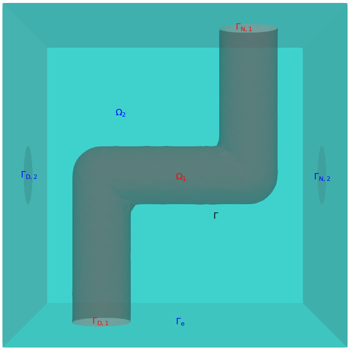
The true domain: a pipe separating the cold fluid from the hot one.
We want to optimize the shape of the pipe connecting the inlet to the outlet of \(\Omega_1\) in order to maximize the heat exchanged between the fluids under two constraints: firstly, the volume of the pipe is prescribed, and secondly, the pressure drop seen from the angle of the energy dissipated by the fluid must remain below a prescribed threshold.
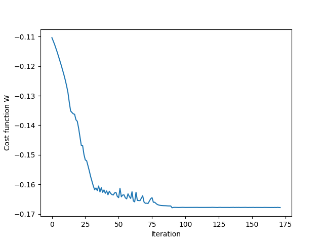
To work with a minimization problem, we define the negative heat exchanged \(W\) as
\[
W(\Gamma) = \int_{\Omega_1} \boldsymbol{u}_1 \cdot \nabla \mathsf{T}_1 \, \mathrm{d}x - \int_{\Omega_2} \boldsymbol{u}_2 \cdot \nabla \mathsf{T}_2 \, \mathrm{d}x,
\]
where \(\boldsymbol{u}_i\) and \(\mathsf{T}_i\), \(i=1,2\), denote the respective solutions of the above problems.
%
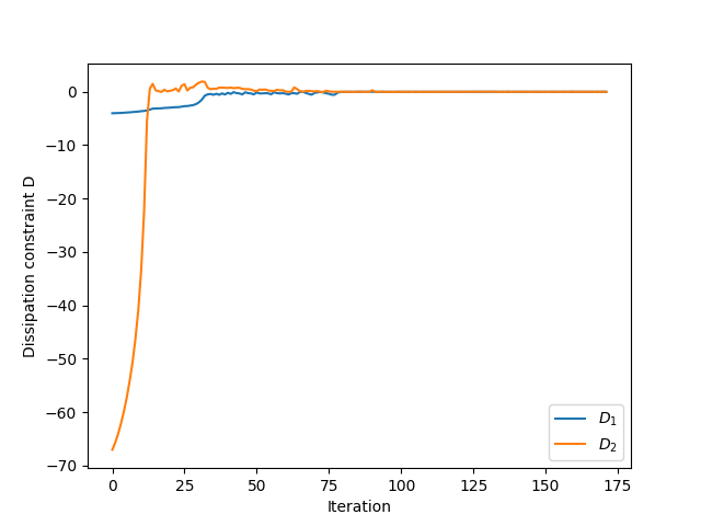
We consider three constraints: firstly the energy dissipation \(D_i\), with a given threshold \(D_{0,i} > 0\) in the fluid labelled by \(i\), defined as
\[
D_i(\Gamma) = \int_{\Omega_i} 2 \nu_i |\varepsilon(\boldsymbol{u}_i)|^2 \, \mathrm{d}x - D_{0,i}, \qquad i=1,2,
\]
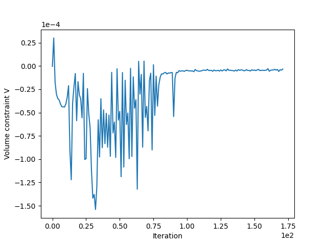
and secondly the gap between the volume occupied by the hot fluid and a target volume \(V_0 > 0\) given by
\[V(\Gamma) = \int_{\Omega_1} 1 \, \mathrm{d}x - V_0.
\]
%
The problem that we consider in this article is the following:
\[
\inf_{\Gamma} W(\Gamma)
\quad \text{ such that } \quad D_i(\Gamma) \leq 0, \, i=1,2, \quad \mbox{ and } \quad V(\Gamma) = 0.
\]
Contributions.
Use of an asymptotic model for the temperature.
The pipe wall is assummed thick.
In order to avoid a mesh at the size of this small parameter, the pipe's wall are modelled thanks to a non standard
interface condition involving second order tangential derivatives: the original problem set in three materials is replaced by the two domains problem
\[ \left\{\begin{array}{rcll}
-\text{div}(\kappa_1 \nabla \mathsf{T}_1) + \boldsymbol{u} \cdot \nabla \mathsf{T}_1 & = & 0
& \text{ in } \Omega_{1}, \\[4pt]
-\text{div}(\kappa_2 \nabla \mathsf{T}_2 ) & = & 0 & \text{ in } \Omega_2, \\[4pt]
\mathsf{T}_1 & = & \mathsf{T}_{\mathrm{D}} & \text{ on } \Gamma_{\mathrm{D}}, \\[4pt]
\displaystyle{\kappa_1 \frac{\partial \mathsf{T}_1}{\partial \boldsymbol{n}} } & = & 0 & \text{ on } \Gamma_{\mathrm{N}}, \\[4pt]
% \displaystyle{\kappa_2 \frac{\partial \mathsf{T}_2}{\partial \boldsymbol{n}} } & = & \color{magenta}0 & \color{magenta}\text{ on } \Gamma_{\mathrm{e,N}}, \\[4pt]
\displaystyle{\kappa_2 \frac{\partial \mathsf{T}_2}{\partial \boldsymbol{n}} + \alpha \mathsf{T}_2} & = & \alpha {\mathsf{T}_{\rm ext}} & \text{ on } \Gamma_{\mathrm{R}}, \\[6pt]
\displaystyle{\left < \kappa \frac{\partial \mathsf{T}}{\partial \boldsymbol{n}}\right >} & = & -\kappa_{\mathrm{m}} \epsilon^{-1} \left [\mathsf{T} \right] & \text{ on } \Gamma, \\[8pt]
\displaystyle{\left [ \kappa \frac{\partial \mathsf{T}}{\partial \boldsymbol{n}} \right]} & = & \epsilon \text{div}_\tau(\kappa_{\mathrm{m}} \nabla_\tau \langle \mathsf{T} \rangle) - \kappa_{\mathrm{m}} H [\mathsf{T}] & \text{ on } \Gamma,\\[8pt]
\displaystyle{\kappa_i \frac{\partial \mathsf{T}_i}{\partial \boldsymbol{n}}} & = & 0 & \text{ on } \partial \Gamma, i=1,2 ,
\end{array} \right.
\]
where \( [u] \) is the jump of \(u\) and \(< u>\) its mean across the interface.
Derivation of shape derivative.
See the paper for the expressions.
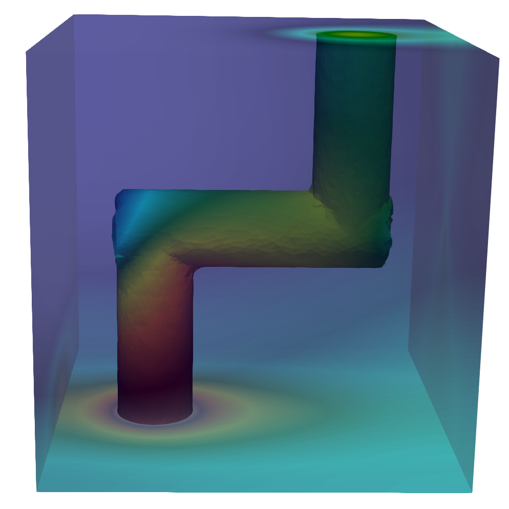
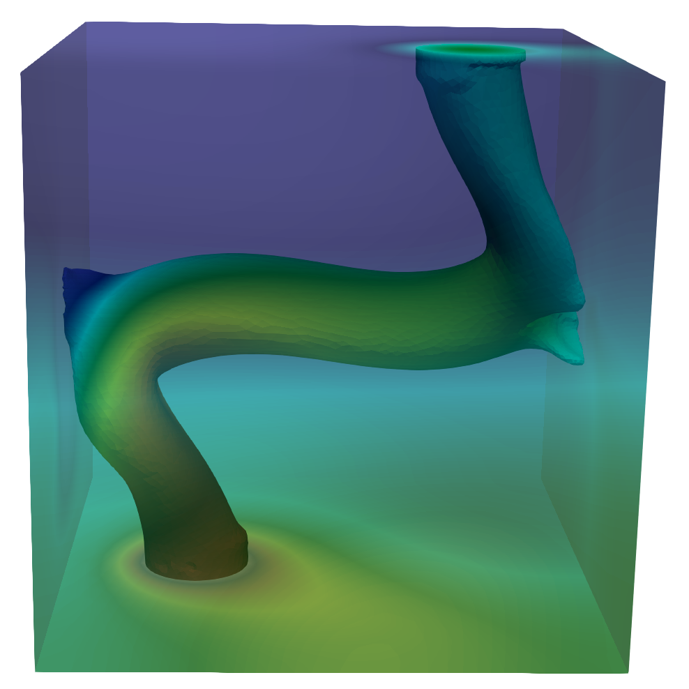
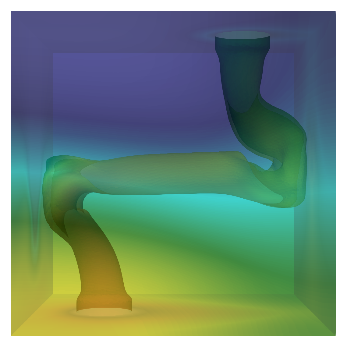
Numerical results
Temperature distribution in: Left: initial shape Center: after 30 iterations Right: after 100 iterations. Evolution of: Left: the objective \(W\) Center : violation of the dissipation constraints \(D_1\) and \(D_2\)
Right: violation of the volume constraint.