Fabien Caubet, Carlos Conca, Marc Dambrine, Rodrigo Zelada. How to insulate a pipe? HAL hal-04772321
Problem statement.
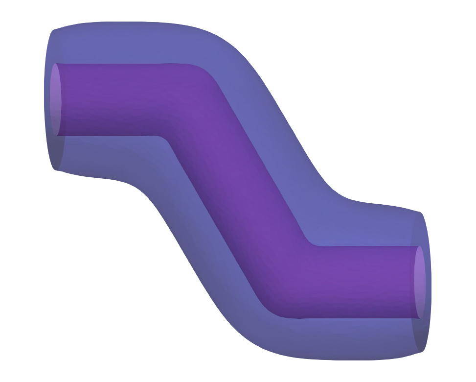
We are interested in the optimal insulation of a pipe where hot water runs.
As the pipe may have a complex geometry, the flow of the hot fluid is described by the stationary incompressible
Navier-Stokes equations.
\[\displaystyle{\left \{ \begin{array}{rll}
-\nu \Delta \boldsymbol{u}^\epsilon + (\nabla \boldsymbol{u}^\epsilon )\boldsymbol{u}^\epsilon + {\dfrac{1}{\rho}}\nabla p^\epsilon & = 0
& \text{ in } \Omega_{1}^\epsilon, \\
\text{div}(\boldsymbol{u}^\epsilon) & = 0 & \text{ in } \Omega_{1}^\epsilon, \\
\boldsymbol{u}^\epsilon & = \boldsymbol{u}_{\mathrm{D}} & \text{ on } \Gamma_{\mathrm{D}} ^\epsilon, \\
\sigma(\boldsymbol{u}^\epsilon,p^\epsilon)\boldsymbol{n} & = 0 & \text{ on } \Gamma_{\mathrm{N}} ^\epsilon, \\
\boldsymbol{u}^\epsilon & = 0 & \text{ on } \Gamma_1 ^\epsilon,
\end{array} \right.}\]
We consider the following shape optimization problem: given a prescribed volume~\(V_0 >0\) of insulating material,
minimize the criterion \(J\) by
\[
J(\Omega_2) = \int_{\Gamma_{\mathrm{R}}} \left(\kappa_2 \frac{\partial \mathsf{T}_2}{\partial \boldsymbol{n}} \right)^2 \,
\mathrm{d}s =\int_{\Gamma_{\mathrm{R}} } \alpha^2 (\mathsf{T}_2 - {\mathsf{T}_{\rm ext}})^2 \, \mathrm{d}s ,
\]
where the temperature \(\mathsf{T}\) solves the approximate convection-diffusion problem
and the fluid speed solves the Navier-Stokes system.
Contributions.
Use of an asymptotic model for the temperature.
The pipe wall is assummed thick.
In order to avoid a mesh at the size of this small parameter, the pipe's wall are modelled thanks to a non standard
interface condition involving second order tangential derivatives: the original problem set in three materials is replaced by the two domains problem
\[ \left\{\begin{array}{rcll}
-\text{div}(\kappa_1 \nabla \mathsf{T}_1) + \boldsymbol{u} \cdot \nabla \mathsf{T}_1 & = & 0
& \text{ in } \Omega_{1}, \\[4pt]
-\text{div}(\kappa_2 \nabla \mathsf{T}_2 ) & = & 0 & \text{ in } \Omega_2, \\[4pt]
\mathsf{T}_1 & = & \mathsf{T}_{\mathrm{D}} & \text{ on } \Gamma_{\mathrm{D}}, \\[4pt]
\displaystyle{\kappa_1 \frac{\partial \mathsf{T}_1}{\partial \boldsymbol{n}} } & = & 0 & \text{ on } \Gamma_{\mathrm{N}}, \\[4pt]
% \displaystyle{\kappa_2 \frac{\partial \mathsf{T}_2}{\partial \boldsymbol{n}} } & = & \color{magenta}0 & \color{magenta}\text{ on } \Gamma_{\mathrm{e,N}}, \\[4pt]
\displaystyle{\kappa_2 \frac{\partial \mathsf{T}_2}{\partial \boldsymbol{n}} + \alpha \mathsf{T}_2} & = & \alpha {\mathsf{T}_{\rm ext}} & \text{ on } \Gamma_{\mathrm{R}}, \\[6pt]
\displaystyle{\left < \kappa \frac{\partial \mathsf{T}}{\partial \boldsymbol{n}}\right >} & = & -\kappa_{\mathrm{m}} \epsilon^{-1} \left [\mathsf{T} \right] & \text{ on } \Gamma, \\[8pt]
\displaystyle{\left [ \kappa \frac{\partial \mathsf{T}}{\partial \boldsymbol{n}} \right]} & = & \epsilon \text{div}_\tau(\kappa_{\mathrm{m}} \nabla_\tau \langle \mathsf{T} \rangle) - \kappa_{\mathrm{m}} H [\mathsf{T}] & \text{ on } \Gamma,\\[8pt]
\displaystyle{\kappa_i \frac{\partial \mathsf{T}_i}{\partial \boldsymbol{n}}} & = & 0 & \text{ on } \partial \Gamma, i=1,2 ,
\end{array} \right.
\]
where \( [u] \) is the jump of \(u\) and \(< u>\) its mean across the interface.
The computational domain for the temperature.
Derivation of shape derivative.
See the paper for the expressions.
Numerical results
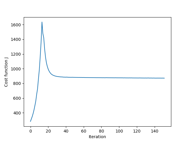
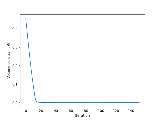
Left: initial shape with exceeding insulating material Right: after 150 iterations. Left: evolution of the objective Right: evolution of the constraint.